|
|
This section includes illustrations of three situations where relative value indicators would improve decision-making.
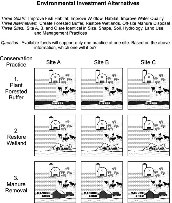
The purpose of the illustrations presented in this section is limited to a) showing how landscape factors affect relative ecosystem values, and b) showing how indicators of relative values based on landscape context should affect decisions about conserving or restoring ecosystems. Actual indicators of relative value are not provided as part of these illustrations. Ongoing work is defining and testing indicators that could be used in each of the three circumstances described. Developing a decision-support system that would be credible and easy to use will require considerable work. The purpose of presenting the illustrations is to provide prospective users with a basis for determining if that work would be worthwhile. Future work will employ indicators into simple web-based decision-support tools. These tools will employ standard indicator definitions and regional geographic information systems (GIS) in ways that allow users to compare environmental investment alternatives using a five step process: 1) Enter the locations of two or more sites being considered (e.g., lat./long. coordinates), 2) Specify the change in site conditions being considered (e.g., conservation practice), 3) Compare default measures of relative value indices. 4) Examine assumptions used, and override where justified, and 5) Evaluate results and adjust to account for special circumstances. Illustration #1: Comparing Conservation Practices Reconsider the environmental investment options depicted in figures 1 and 2. Again assume that you have been asked to compare the potential benefits of the nine alternatives (3 sites and 3 conservation practices). This time lets focus on assessing potential benefits with respect to three specific outcomes: water quality , in-stream fish habitat, and terrestrial wildlife habitat.
Figure 1 Again, all of the projects may be worthwhile. However, with funding to support only one alternative and similar costs for each alternative the critical question is:
There are two sets of information that can be used to address this question: information about site conditions and information about offsite conditions. site criteria In order to focus the illustration the three farm sites are shown in Figure 1 to be identical in terms of size, shape, and land use. Assume also that they are identical in terms of soil, slope, hydrology, vegetative cover, and all other biophysical characteristics. Based on site information alone, therefore, it is not possible to predict any differences in the expected benefits from investing at any of the three sites. The Conservation Practices Physical Effects or CPPE model used to assess some USDA spending decisions might be used here to identify which of the three practices is likely to have physical effects that could improve fish and wildlife habitat and water quality. However, CPPE provides no basis for judging why one project or one site should be preferred over another. Let's consider how the landscape differences depicted in Figure 2 can be used to compare the expected environmental payoffs from investing in each of the project alternatives at each of the sites. landscape criteria
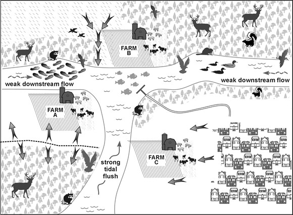
Figure 2 Figure 2 provides a bird's eye view of the watershed, showing the three farms relationship to the landscape. Various symbols are used to show the proximity of the three farm sites to fish and wildlife habitats, to people, and to several types of water bodies. The yellow arrows depict the direction of surface water and agricultural runoff. As described in previous sections the position of the sites with respect to various landscape features either limit or enhance the capacity of the site to provide certain environmental functions. It also influences the level of environmental services they will generate and how valuable they will be to people. This provides a useful focus for developing environmental benefit indicators. Important factors include: the type and condition of the nearby water body, the site's proximity and connectivity to natural and man-made landscape features, the accessibility of the site to fish and wildlife, and to people, the availability of substitute habitats for fish and wildlife, alternative recreation or viewing areas, risk factors related to the potential biological, physical, and chemical threats to the site, and so on. Consider how differences in the landscape context of the three sites depicted in Figure 2 might affect the level of expected benefits with respect to each of the three benefit categories identified earlier. Water Quality Benefits All three sites are adjacent to rivers and investing in wetlands or riparian buffers at any of them would have the potential to trap sediment and nutrient runoff. However, the sites differ in terms of the quantity and quality of runoff received, the types of receiving waters, and the resources at-risk from runoff. Because of topography, only a small amount of runoff traverses Site A before reaching the water body, so benefits would be limited to reducing on-farm runoff to the downstream habitat. The runoff from Site B, on the other hand, is an accumulation of runoff from several farms and is delivered to a slow moving stream that is near shellfish and finfish habitats where it poses a clear threat. The finfish habitat is accessible by a fishing pier so the benefits from providing fish habitat are local and apparent At Site C, runoff from the farm and upslope septic fields reaches the main stem of the river that is fast moving and has a strong tidal flush, so effects to the nearby shellfish bed are less certain. It is likely that most benefits would accrue in the downstream estuary or near-coastal environment. Farm C is also providing valuable views of the river to the adjacent houses, so a forested buffer could reduce housing values. Based on what is shown in Figure 2 investments at Site B would provide the most water quality benefits followed by Site C (non-forested buffer) and then Site A. Fishery-Related Benefits Wetlands contribute directly to fish habitat by providing feeding and breeding areas for fish and forage species. Aside from water quality improvements, wetland restoration is the only one of the three conservation practices that contributes to improved fish habitat. Site C is downstream of the only fish habitat depicted in Figure 2, so investing in wetlands at that site would not have any significant affect on fish habitat. Because of its location, Site A has only a nominal influence on the stream habitat. Based on the information provided in Figure 2, investing in wetland restoration at Site B is the only alternative that would result in direct fishery-related benefits. Note that the residents of the development near Site C and across the river from Site B have direct access to finfish and shellfish areas protected by Site B. Wildlife-Related Benefits Site B is adjacent to healthy wildlife habitats on the left and on the right and provides a critical corridor between them. By contrast, the wildlife habitat near Site C is scanty and a road blocks the corridor between it and Site C. The wildlife habitat near Site A is also less significant and a wetland or buffer constructed there would not connect that habitat to any other habitat. Site B clearly provides greater wildlife benefits than the other two sites. Note that offsite manure disposal, although perhaps the most direct way of providing water quality benefits at all three sites, would provide no direct fish or wildlife benefits. Outcome of Illustration The benefits from applying conservation practices at a particular site will usually be impossible to measure in terms of dollars. It may also be impossible to trace environmental improvements that result in benefits to specific conservation practices or USDA spending decisions. Nonetheless, the benefits that result from conservation practices applied in different regions and at different sites can differ widely. To achieve the greatest environmental benefits per dollar spent, these differences need to be taken into account in project eligibility and ranking criteria. This section describes conservation benefit indicators that can be used to assess and compare the expected payoffs from investing in conservation practices undertaken at different sites. Illustration 2: Wetland Trading Figure
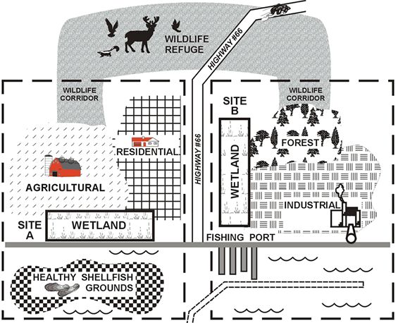
3 depicts two wetlands that are identical in terms of size and shape.
Assume also that they are identical in terms of biophysical characteristics
(e.g., soil, hydrology, and vegetative cover). Consider a trade
between a wetland at Site A and Site B., perhaps in a mitigation context,
and compare gains and losses with respect to three specific functions:
wildlife habitat, fishery support, and water quality. Since the biophysical
features of wetlands at both sites are identical the gains and losses
in wetland capacity to provide all three functions would be identical.
However, because Site A is in a different landscape context the losses
in wetland values can be expected to be significantly greater than the
gains. This is the case because:
Figure 3 To make Site A seem even more valuable, Figure 3 also depicts Site A where it provides aesthetic and educational opportunities to a nearby residential population whereas Site B is surrounded by industrial sites and private forest lands which limits its amenity values. To be even more sure that the relative value of Site A is greater than Site B, consider differences in the exposure of the two sites to natural and man-made risks that could disrupt the flow of beneficial services from the two sites. For example, assume that a new 10-year land use plan for the region designates the area around Site A as environmentally sensitive, no industrial uses whereas the area around Site B as industrial use, fast-track permitting. Not only are the current environmental values provided at Site A higher than those provided by Site B, they are less likely to be decline in the future as a result of land use changes. The same type of differences in site risks might be associated with the exposure and vulnerability of the two sites to threats from water diversion, sea level rise, invasive species, or other factors. Based purely on the geographic information presented in Figure 3, it is possible to pose a technically and legally defensible argument that a wetland at Site A is more valuable than an identical wetland at Site B. This demonstrates the logic of the indicator system that we outline in the following section, which relies on geographic information systems (GIS) to compare ecosystem value. Without judging the merits of protecting or improving wetland capacity at both Site A and Site B, the illustration shows that indicators can be used to reflect important valuation tradeoffs without resorting to conventional (dollar-based) valuation. Now examine how this would be reflected in indicators of relative wetland values. Using Indicators to "Score" a Wetland Trade Assume
that each of the indicators described in the previous section are designed
to range around a mean or average value of one. At a site in a landscape
context that is average in every way, for example, an increase in functional
capacity of 10% would be expected to result in a similar 10% increase
in expected levels of function, service, and value. (.1 X 1 X 1 X 1= .1)
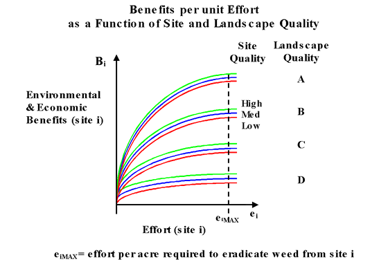
Now consider Site A and Site B in Figure 3 and assume that Site A is in a location that is 20% above average in every way and that Site B is in a location that is 20% below average in every way. Since we assumed that the size, shape, and biophysical characteristics of Site A and Site B are the same they would rank the same in terms of functional capacity, and an investment to achieve a 10% increase in functional capacity at both sites would yield the same onsite results and cost about the same. However, because Site A is 20% above average in every way, a 10% increase in functional capacity at that site would result in a 12% increase in function, a 14% increase in service, and a 17.3% increase in value (.1 X 1.2 X 1.2 X 1.2 = .173) (see Figures 4 and Figure 5). Similarly, since Site B is 20% below average in every way the same 10% increase in onsite functional capacity would result in only an 8% increase in function, a 6.4% increase in service, and a 5.1% increase in value (.1 X .8 X .8 X .8 =5.1).Ê This implies that investments aimed at improving functional capacity at Site A would result in 340% more economic value than similar investment at Site B. It also implies that allowing wetland mitigation trading that involved gaining an acre of wetland at Site B and losing an acre of wetland at Site A would result in an economic loss of 340% even though the sites themselves are identical. Value-based analyses such as this could support significant changes in the way ecosystems are compared. In the case of wetland mitigation trading, for example, gains and losses are frequently scored using area measures or biophysical measures that reflect functional capacity. In such instances, wetland acreage at Site A and Site B in Figure 3 would be considered an even trade. However, if trading rules were designed to achieve no net loss of wetland value, the trading rules, based on the indicator system outlined above, would require a "compensation ratio" of at least 3 or 4 acres of wetlands at Site B to compensate for each 1 acre of wetland lost at Site A. Illustration # 3- Eradicating Noxious Weeds The application of site based ecosystem value indicators to guide spending on invasive weed management is illustrated in Figure 6. The effect of the weed infestation at an ecosystem site is characterized as a reduction in functional capacity which increases as effort is increased to remove the weed. Assume that the level of infestation and the cost of treatment are the same at all sites and that budget constraints limit the number of sites that can be treated. The payoff from treating a site depends on the level of functional capacity at the site in the absence of weeds, which is indicated in Figure 4 as low, medium and high. However, the payoff also depends on the landscape context of the sites indicated in Figure 6 as A, B, C or D, where A reflects an extremely high quality landscape context (strong indicators) and D reflects a relatively poor landscape context (weak indicators). The level of benefits at all sites depends on the intensity of the effort to control or eradicate weeds, which is reflected by e (effort). However, it is also affected by site and landscape conditions. If the cost per unit effort is the same at all sites, the indicator system can be used to prioritize sites on the basis of expected net economic benefits.
Figure 6 Figure 7 below carries the weed illustration a step further by showing that the expected payoff from controlling weeds at one site depends not only on the level of effort at that site (e.g., spending per hectare), but on the geographic extent of the response (e.g., number of hectares treated). Here again landscape indicators can be used to determine the likelihood that a site that is treated will become reinfested as a result of leaving adjacent or nearby sites untreated. The expected benefits from investing in weed control at a given site, in other words, depends on the level of infestation and the level of treatment at other nearby sites.
Figure 7 In the face of limited budgets, the tradeoffs between increasing spending at the intensive margin (e.g., more effort and spending per hectare) and increasing spending at the extensive margin (e.g., more hectares treated) are extremely important. In an increasing number of areas, the risk posed to functional capacity by invasive species is the most important factor limiting the success of efforts to protect or restore ecosystems. In these areas, leading indicators of the direction, spread rate, and toxicity of invasive species may be the most important non-monetary basis for comparing the value of environmental investments. In our indicator system harmful invasive species affect ecosystem values by changing site and/or landscape characteristics in ways that reduce expected functions, services, and values. An ecosystem site that achieves high value indices based on current site and landscape conditions but faces an uncontrolled threat from invasive species may be far less valuable than a site with a lower current value that is either not threatened by invasives or is facing a threat that is being addressed.  |