|
       
|
Definitions in this text:

Methods, Section 4
Travel Cost Method
- Overview
- Hypothetical Situation
- Why Use the Travel Cost Method
- Options for Applying the Travel Cost Method
- Application of the Zonal Travel Cost Approach
- Application of the Individual Travel Cost Approach
- Application of the Random Utility Approach
- Case Study Examples of the Travel Cost Valuation
- Case # 1¡¦Environmental Conservation
- Case # 2¡¦Improvements in Water Quality
- Summary of the Travel Cost Method
- Applying the Travel Cost Method
- Advantages of the Travel Cost Method
- Issues and Limitations
The travel cost method is used to estimate economic use values associated with ecosystems or sites that are used for recreation.
The method can be used to estimate the economic benefits or costs resulting from:
- changes in access costs for a recreational site
- elimination of an existing recreational site
- addition of a new recreational site
- changes in environmental quality at a recreational site
This section continues with some example applications of the travel cost method, followed by a more complete technical description of the method and its advantages and limitations.
A site used mainly for recreational fishing
is threatened by development in the surrounding area. Pollution and
other impacts from this development could destroy the fish habitat at the
site, resulting in a serious decline in, or total loss of, the site¡¦s ability
to provide recreational fishing services. Resource agency staff want
to determine the value of programs or actions to protect fish habitat at
the site.
Why Use the Travel Cost Method?
The travel cost method was selected in this case for two main reasons:
- 1. The site is primarily valuable to people
as a recreational site. There are no endangered species or other
highly unique qualities that would make non-use values for the site significant.
2. The expenditures for projects to protect the site are relatively low. Thus, using a relatively inexpensive method like travel cost makes the most sense.
Alternative Approaches:
Contingent valuation or contingent choice
methods could also be used in this case. While they might produce
more precise estimates of values for specific characteristics of the site,
and also could capture non-use values, they would be considerably more
complicated and expensive to apply.
Options for Applying the Travel Cost
Method:
There are several ways to approach the problem, using variations of the travel cost method.
These include:
- A simple zonal travel cost approach, using mostly secondary data, with some simple data collected from visitors.
- An individual travel cost approach, using a more detailed survey of visitors.
- A random utility approach using survey and other data, and more complicated statistical techniques.
Application of the Zonal Travel Cost Approach:
The zonal travel cost method is the simplest and least expensive approach. It will estimate a value for recreational services of the site as a whole. It cannot easily be used to value a change in quality of recreation for a site, and may not consider some of the factors that may be important determinants of value.
The zonal travel cost method is applied by collecting information on the number of visits to the site from different distances. Because the travel and time costs will increase with distance, this information allows the researcher to calculate the number of visits ¡¦purchased¡¦ at different ¡¦prices.¡¦ This information is used to construct the demand function for the site, and estimate the consumer surplus , or economic benefits, for the recreational services of the site.
Step 1:
The first step is to define a set of zones
surrounding the site. These may be defined by concentric circles
around the site, or by geographic divisions that make sense, such as metropolitan
areas or counties surrounding the site at different distances.
Step 2:
The second step is to collect information
on the number of visitors from each zone, and the number of visits made
in the last year. For this hypothetical example, assume that staff
at the site keep records of the number of visitors and their zipcode, which
can be used to calculate total visits per zone over the last year.
Step 3:
The third step is to calculate the visitation
rates per 1000 population in each zone. This is simply the total
visits per year from the zone, divided by the zone¡¦s population in thousands.
An example is shown in the table:
|
|
|
|
|
|
|
|
|
|
|
|
|
|
|
|
|
|
|
|
|
|
|
|
|
|
|
|
||
|
|
|
Step 4:
The fourth step is to calculate the average
round-trip travel distance and travel time to the site for each zone.
Assume that people in Zone 0 have zero travel distance and time.
Each other zone will have an increasing travel time and distance.
Next, using average cost per mile and per hour of travel time, the researcher
can calculate the travel cost per trip. A standard cost per mile
for operating an automobile is readily available from AAA or other sources.
Assume that this cost per mile is $.30. The cost of time is more
complicated. The simplest approach is to use the average hourly wage.
Assume that it is $9/hour, or $.15/minute, for all zones, although in practice
it is likely to differ by zone. The calculations are shown in the
table:
|
|
Travel Distance |
Travel Time |
|
|
|
|
|
|
|
|
|
|
|
|
|
|
|
|
|
|
|
|
|
|
|
|
|
|
|
|
|
|
|
Step 5:
The fifth step is to estimate, using regression analysis, the equation that relates visits per capita to travel costs and other important variables. From this, the researcher can estimate the demand function for the average visitor. In this simple model, the analysis might include demographic variables, such as age, income, gender, and education levels, using the average values for each zone. To maintain the simplest possible model, calculating the equation with only the travel cost and visits/1000, Visits/1000 = 330 ¡¦ 7.755*(Travel Cost).
Step 6:
The sixth step is to construct the demand function for visits to the site, using the results of the regression analysis. The first point on the demand curve is the total visitors to the site at current access costs (assuming there is no entry fee for the site), which in this example is 1600 visits per year. The other points are found by estimating the number of visitors with different hypothetical entrance fees (assuming that an entrance fee is viewed in the same way as travel costs).
For the purposes of our example, start
by assuming a $10 entrance fee. Plugging this into the estimated
regression equation, V = 330 ¡¦ 7.755C, gives the following:
|
|
|
|
|
|
|
|
|
|
|
|
|
|
|
|
|
|
|
|
|
|
|
|
|
|
|
|
|
|
|
Total Visits
|
|
This gives the second point on the demand
curve¡¦954 visits at an entry fee of $10. In the same way, the number
of visits for increasing entry fees can be calculated, to get:
|
|
|
|
|
|
|
|
|
|
|
|
|
|
|
These points give the demand curve for trips to the site.
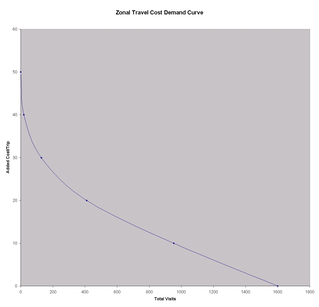
Step 7:
The final step is to estimate the total economic benefit of the site to visitors by calculating the consumer surplus, or the area under the demand curve. This results in a total estimate of economic benefits from recreational uses of the site of around $23,000 per year, or around $14.38 per visit ($23,000/1,600).
How Do We Use the Results?
Remember that the agency staff¡¦s objective
was to decide whether it is worthwhile to spend money on programs and actions
to protect this site. If the actions cost less than $23,000 per year,
the cost will be less than the benefits provided by the site. If
the costs are greater than this, the staff will have to decide whether
other factors make them worthwhile.
Application of the Individual Travel Cost Approach:
The individual travel cost approach is similar to the zonal approach, but uses survey data from individual visitors in the statistical analysis, rather than data from each zone. This method thus requires more data collection and slightly more complicated analysis, but will give more precise results.
For the hypothetical example of the recreational fishing site, rather than simply collecting information on number of visitors and their zipcodes, the researcher would conduct a survey of visitors. The survey might ask for the following information:
- location of the visitor¡¦s home ¡¦ how far they traveled to the site
- how many times they visited the site in the past year or season
- the length of the trip
- the amount of time spent at the site
- travel expenses
- the person¡¦s income or other information on the value of their time
- other socioeconomic characteristics of the visitor
- other locations visited during the same trip, and amount of time spent at each
- other reasons for the trip (is the trip only to visit the site, or for several purposes)
- fishing success at the site (how many fish caught on each trip)
- perceptions of environmental quality or quality of fishing at the site
- substitute sites that the person might visit instead of this site
Because additional data about visitors, substitute sites, and quality of the site has been collected, the value estimates can be ¡¦fine tuned¡¦ by adding these other factors to the statistical model. Including information about the quality of the site allows the researcher to estimate the change in value of the site if its quality changes. To do so, two different demand curves would be estimated¡¦one for each level of quality. The area between these two curves is the estimate of the change in consumer surplus when quality changes.
In the example, the researcher might recognize
that development around the site is unlikely to totally destroy the fish
population. However, it could diminish the population enough to adversely
affect catch rates. By including catch rates in the model, the researcher
can estimate the lost recreational benefits from reduced catch rates.
However, the random utility model, described in the next section, is a
more appropriate approach for this type of estimation.
Application of the Random Utility Approach:
The random utility approach is the most complicated and expensive of the travel cost approaches. It is also the ¡¦state of the art¡¦ approach, because it allows for much more flexibility in calculating benefits. It is the best approach to use to estimate benefits for specific characteristics, or quality changes, of sites, rather than for the site as a whole. It is also the most appropriate approach when there are many substitute sites.
In the example, the agency might want to value the economic losses from a decrease in fish populations, rather than from loss of the entire fish stock. The random utility approach would be the best way to do so, because it focuses on choices among alternative sites, which have different quality characteristics.
The random utility approach assumes that individuals will pick the site that they prefer, out of all possible fishing sites. Individuals make tradeoffs between site quality and the price of travel to the site. Hence, this model requires information on all possible sites that a visitor might select, their quality characteristics, and the travel costs to each site.
For the example, the researcher might conduct a telephone survey of randomly selected residents of the state. The survey would ask them if they go fishing or not. If they do, it would then ask a series of questions about how many fishing trips they took over the last year (or season), where they went, the distance to each site, and other information similar to the information collected in our individual travel cost survey. The survey might also ask questions about fish species targeted on each trip, and how many fish were caught.
Using this information, the researcher can estimate a statistical model that can predict both the choice to go fishing or not, and the factors that determine which site is selected. If quality characteristics of sites are included, the model can easily estimate values for changes in site quality, for example the economic losses caused by a decrease in catch rates at the site.
Case Study Examples of the Travel Cost
Method:
Case # 1¡¦Environmental Conservation
The Situation
Hell Canyon on the Snake River separating
Oregon and Idaho offers spectacular vistas and outdoor amenities to visitors
from around the country and supports important fish and wildlife habitat.
It also has economic potential as a site to develop hydropower. Generating
hydropower there would require building a dam behind which would form a
large lake. The dam and the resulting lake would significantly and permanently
alter the ecological and aesthetic characteristics of Hell Canyon.
The Challenge
During the 1970¡¦s, there were major controversies
regarding the future of Hell Canyon. Environmental economists from Resources
For The Future in Washington, D.C. were asked to develop an economic analysis
to justify preserving Hell Canyon in its natural state in the face of its
obvious economic potential as a source of hydropower.
The Analysis
Researchers estimated that the net economic
value (cost savings) of producing hydropower at Hell Canyon was $80,000
higher than at the "next best" site which was not environmentally sensitive.
They then conducted a low-cost/low precision travel-cost survey to estimate
the recreational value of Hell Canyon and concluded that it was about $900,000.
The researchers did not attempt to strongly defend the "scientific" credibility
of the valuation method they used or the results. However, at public hearings,
they emphasized that, even if the "true value" of recreation at Hell Canyon
was ten times less than their estimate, it would still be greater than
the $80,000 economic payoff from generating power there as opposed to the
other site. They also illustrated that overall demand for outdoor recreation,
for which the supply is limited, was going up, while many other sources
of energy are available besides Hell Canyon hydropower.
The Results
Based largely on the results of this non-market
valuation study, Congress voted to prohibit further development of Hell
Canyon.
Case # 2¡¦Improvements in Water Quality
The Situation
The costs to farmers and taxpayers of
implementing on-farm best management practices to reduce sediment and nutrient
runoff to the Chesapeake Bay are well known. Controversies arose during
the 1980¡¦s, which continue today, over the benefits of resulting improvements
in water quality.
The Challenge
Economists were asked to assess the economic
benefits of water quality improvements to beach users in the Chesapeake
Bay area. They needed to establish linkages between differences in water
quality and differences in willingness to pay for beach use. The hypothesis
that to be tested was that average willingness to pay, as reflected in
the travel costs to visitors to particular beaches, was positively correlated
with water quality. If the hypothesis was correct the empirical results
would allow researchers to estimate the increase in willingness to pay
of improving water quality at all beaches.
The Analysis
Researchers selected the concentration
of nitrogen and phosphorous in the water at the monitoring station nearest
to the beach as an index of water quality at the beach. This was assumed
to reflect the level of objectionable visual and other characteristics
that affect the value of beach use. A cross-sectional analysis of
travel cost data collected from 484 people at 11 public beaches was used
to impute the aggregate willingness to pay for a 20% increase in water
quality, which was assumed to be associated with a 20% reduction in total
nitrogen and phosphorus.
The Results
The average annual benefits to all Maryland
beach users of the improvements in water quality were estimated to be $35
million in 1984 dollars. These were thought to be conservative for
several reasons, including:
- The value of improvements in water quality was only shown to increase the value of current beach use. However, improved water quality can also be expected to increase overall beach use.
- Estimates ignore visitors from outside the Baltimore-Washington statistical metropolitan sampling area.
- The population and incomes in origin zones near the Chesapeake Bay beach areas are increasing, which is likely to increase visitor-days and thus total willingness to pay.
Summary of the Travel
Cost Method:
The travel cost method is used to estimate the value of recreational benefits generated by ecosystems. It assumes that the value of the site or its recreational services is reflected in how much people are willing to pay to get there. It is referred to as a ¡¦revealed preference¡¦ method, because it uses actual behavior and choices to infer values. Thus, peoples¡¦ preferences are revealed by their choices.
The basic premise of the travel cost method is that the time and travel cost expenses that people incur to visit a site represent the ¡¦price¡¦ of access to the site. Thus, peoples¡¦ willingness to pay to visit the site can be estimated based on the number of trips that people make at different travel costs. This is analogous to estimating peoples¡¦ willingness to pay for a marketed good based on the quantity demanded at different prices.
The travel cost method can be used to estimate the economic benefits or costs resulting from:
- changes in access costs for a recreational site
- elimination of an existing recreational site
- addition of a new recreational site
- changes in environmental quality at a recreational site
Applying the Travel Cost Method:
On average, people who live farther from a site will visit it less often, because it costs more in terms of actual travel costs and time to reach the site. The number of visits from origin zones at different distances from the site, and travel cost from each zone, are used to derive an aggregate demand curve for visits to the site, and thus for the recreational or scenic services of the site. This demand curve shows how many visits people would make at various travel cost prices, and is used to estimate the willingness to pay for people who visit the site (whether they are charged an admission fee or not).
Other factors may also affect the number of visits to a site. People with higher incomes will usually make more trips. If there are more alternative sites, or substitutes, a person will make less trips. Factors like personal interest in the type of site, or level of recreational experience will affect the number of visits. A more thorough application will take these and other factors into account in the statistical model.
To apply the travel cost method, information must be collected about:
- number of visits from each origin zone (usually defined by zipcode)
- demographic information about people from each zone
- round-trip mileage from each zone
- travel costs per mile
- the value of time spent traveling, or the opportunity cost of travel time
- exact distance that each individual traveled to the site
- exact travel expenses
- the length of the trip
- the amount of time spent at the site
- other locations visited during the same trip, and amount of time spent at each
- substitute sites that the person might visit instead of this site, and the travel distance to each
- other reasons for the trip (is the trip only to visit the site, or for several purposes)
- quality of the recreational experience at the site, and at other similar sites (e.g., fishing success)
- perceptions of environmental quality at the site
- characteristics of the site and other, substitute, sites
The most controversial aspects of the travel
cost method include accounting for the opportunity cost of travel time,
how to handle multi-purpose and multi-destination trips, and the fact that
travel time might not be a cost to some people, but might be part of the
recreational experience.
Advantages of the Travel Cost Method:
- The travel cost method closely mimics the more conventional empirical techniques used by economists to estimate economic values based on market prices.
- The method is based on actual behavior¡¦what people actually do¡¦rather than stated willingness to pay¡¦what people say they would do in a hypothetical situation.
- The method is relatively inexpensive to apply.
- On-site surveys provide opportunities for large sample sizes, as visitors tend to be interested in participating.
- The results are relatively easy to interpret and explain.
- The travel cost method assumes that people perceive and respond to changes in travel costs the same way that they would respond to changes in admission price.
- The most simple models assume that individuals take a trip for a single purpose ¡¦ to visit a specific recreational site. Thus, if a trip has more than one purpose, the value of the site may be overestimated. It can be difficult to apportion the travel costs among the various purposes.
- Defining and measuring the opportunity cost of time, or the value of time spent traveling, can be problematic. Because the time spent traveling could have been used in other ways, it has an "opportunity cost." This should be added to the travel cost, or the value of the site will be underestimated. However, there is no strong consensus on the appropriate measure¡¦the person¡¦s wage rate, or some fraction of the wage rate¡¦and the value chosen can have a large effect on benefit estimates. In addition, if people enjoy the travel itself, then travel time becomes a benefit, not a cost, and the value of the site will be overestimated.
- The availability of substitute sites will affect values. For example, if two people travel the same distance, they are assumed to have the same value. However, if one person has several substitutes available but travels to this site because it is preferred, this person¡¦s value is actually higher. Some of the more complicated models account for the availability of substitutes.
- Those who value certain sites may choose to live nearby. If this is the case, they will have low travel costs, but high values for the site that are not captured by the method.
- Interviewing visitors on site can introduce sampling biases to the analysis.
- Measuring recreational quality, and relating recreational quality to environmental quality can be difficult.
- Standard travel cost approaches provides information about current conditions, but not about gains or losses from anticipated changes in resource conditions.
- In order to estimate the demand function, there needs to be enough difference between distances traveled to affect travel costs and for differences in travel costs to affect the number of trips made. Thus, it is not well suited for sites near major population centers where many visitations may be from "origin zones" that are quite close to one another.
- The travel cost method is limited in its scope of application because it requires user participation. It cannot be used to assign values to on-site environmental features and functions that users of the site do not find valuable. It cannot be used to value off-site values supported by the site. Most importantly, it cannot be used to measure nonuse values. Thus, sites that have unique qualities that are valued by non-users will be undervalued.
- As in all statistical methods, certain statistical problems can affect the results. These include choice of the functional form used to estimate the demand curve, choice of the estimating method, and choice of variables included in the model.
Method 5 - Damage Cost Avoided
Back to:
Method
3 - Hedonic Pricing